


Introduction
GenomicsPortals is a web-based integrative computational platform
for the analysis and mining of genomics data. We aim to integrate
the primary genomics data, functional knowledge base and analytical
tools within a single framework.
Genomics datasets are organized thematically into different portals.
Different portals can contain datasets related to different diseases
(eg Breast Cancer and Prostate Cancer), specific types of genomics
data (eg Epigenomics and Transcription Factors), or different biological
processes (eg Development). The same dataset can be assigned to different
portals.
A typical analysis starts by constructing a list of genes by either
using the predefined lists of pasting a gene list of interest, querying
one of the databases with genome-scale data and producing analysis
summaries. One can also start by searching for dataset of interest,
and then constructing the query gene lists. In this case, one can
also construct gene lists by browsing pre-computed clustering results.
We would like to note that we have designed the layout with the font
size of 16 as a reference. If required, this default font size can
be changed in the browser to increase the readability. In certain
cases, simply ``zoming in'' will also make the text easier to
read without pictures going out of focus.
Start by constructing a gene list
There are many ways to construct a gene list.
- Use a predefined gene list.
- Search for genes of interest using entrez id, symbol or description.
- Paste a list of genes in the box provided.
- Find predefined gene list(s) for your choice of genes.
- Find genes with a phrase in their RIFs.
- Find biogrid gene pairs for your gene(s).
The above list depicts various starting points to generate a list
of genes of your interest. Rest of the work-flow is quite similar
no matter how one selects a gene list.
Using predefined gene list(s)
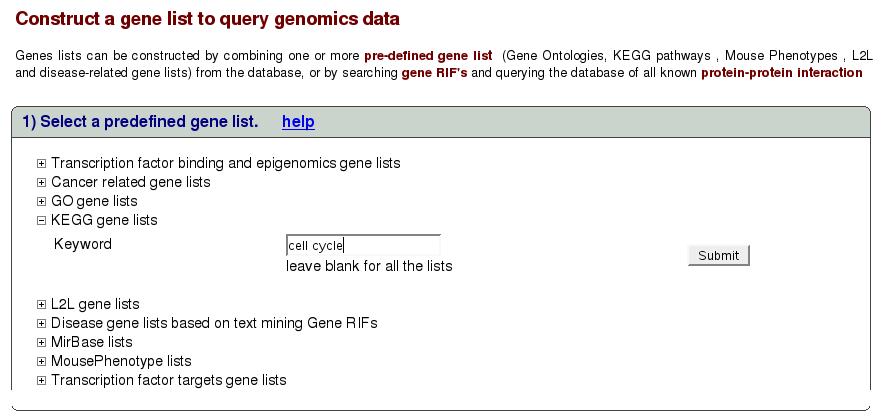
Figure![[*]](crossref.png) shows the interface to select
a predefined gene list. Clicking on ``Gene List'' tab in the left
menu would get this page. The lists are organized in different categories
and we are constantly adding new lists and categories. Let's say we
are interested in gene lists in category ``KEGG'' with keywords
``cell cycle''. Click on the link ``KEGG gene list'' to expand
the search box as shown below. Type cell cycle in the text box and
click submit.
shows the interface to select
a predefined gene list. Clicking on ``Gene List'' tab in the left
menu would get this page. The lists are organized in different categories
and we are constantly adding new lists and categories. Let's say we
are interested in gene lists in category ``KEGG'' with keywords
``cell cycle''. Click on the link ``KEGG gene list'' to expand
the search box as shown below. Type cell cycle in the text box and
click submit.
Figure:
Search a predefined gene list
|
This takes us to the following screen (figure).
Here we see a list of gene list returned for the keywords. Select
one or multiple lists using the check boxes and click submit.
Figure:
Select gene list

|
Now we see summary for the submitted lists. Note that below the summary
table, we are asked to select union or intersection of the gene lists
selected. In this case, because we submitted only one gene list, both
union and intersection are identical. Let's select union and proceed
to select an experiment for analysis.
Figure:
Summary of gene list

|
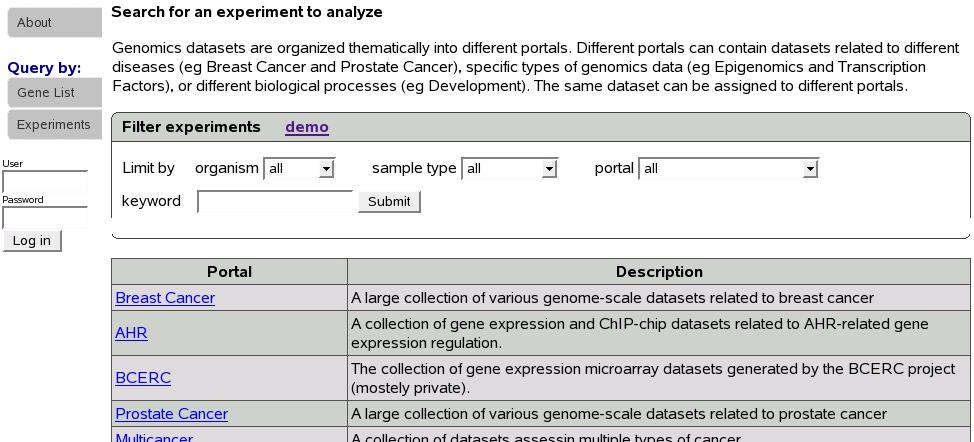
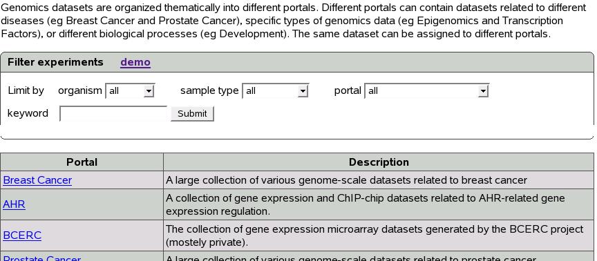
Experiments are organized into different portals. If we know the portal
the experiment of our interest belongs to, we can click on the portal
name to list all the experiments in that portal. Since this is not
the case most times, a search function is provided to look for experiments
of our interest. In the ``Filter experiments'' box shown below,
select organism, sample type, portal of your interest and type in
keyword. Keyword could be left blank.
Figure:
Select or search for experiments
|
Let's click on portal name ``Breastcancer'' to proceed with our
example.
Figure is a part of the screen showing
experiments in the portal Breastcancer. If we had used the search
function to look for an experiment instead, a similar screen would
be shown. Below you would see a list of experiments. Let's select
first experiment (GSE10797) and scroll down and click submit.
Figure:
show experiments

|
At this point, data is retrieved from database for the selected experiment
and gene list(s) as shown in figure.
Figure:
Get data

|
One could download the data for his/her own analysis either as a tab
delimited file or an eset for analysis in R. In this example, we have
66 samples, 209 probes and 103 genes. If we want to analyze only a
subset of samples, we could select samples using the ''Step 1''
shown above. This step is optional and default is to select all the
samples. Next we select a sample grouping for the analysis. We could
choose to cluster on genes, samples, both genes and samples or none
using the combo box shown above. Check the box ``Compute LR''
to compute predictive ability pvalue. Let's select ``CellType''
sample grouping, leave step 1 as it is to select all the samples,
cluster on ``none'' and click Analyze button.
Figure:
Results

|
If we had checked the compute LR box we would see an additional column
``Gene list Statistics'' with the computed pvalue in the results
tables as shown in figure.
Figure:
Results with LR

|
Figure depicts a typical summary table details
of which can be found in Section Interpreting Results'.
Search for genes of interest using entrez
id, symbol or description.
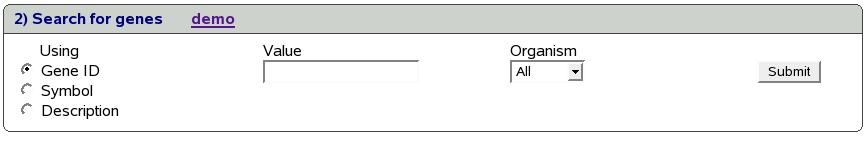
This section describes how to search for genes in the database and
proceed with the analysis of genes found in search results.
Figure:
Search genes
|
Figure shows gene search page. This can be
retrieved by clicking on the ``Gene List'' tab in the left menu.
Genes could be searched by one of the three parameters: Gene ID (Entrez
ID) e.g. 2099, symbol e.g. ``ESR'' or description e.g ``estrogen''.
Type the value in the text box shown above. We can limit the search
to a specific organism if required e.g. human, mouse or rat. For this
example let's search for symbol ``ESR''. To do this, first select
``Symbol'' radio in the left column, type ``ESR'' in the text
box. Select human from the Organism combo box (default is to look
across all organisms) and click submit.
Figure:
Gene search result
|
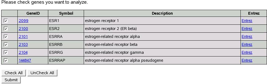
Figure shows the search result. Now we
have all the genes with symbol ``ESR'' or similar symbol names.
To analyze gene(s) select all the genes of interest and then click
submit. Now we are presented a screen to select an experiment to analyze.
From this point on, we proceed as explained in previous section ``Using
predefined gene lists''.
Paste a list of genes in the box provided.
This section describes how to submit your own list of genes for analysis.
Figure:
Submit a custom list of genes
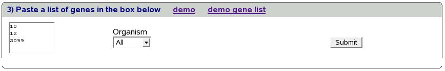
|
Figure shows the screen to submit your own
list of genes. You can use either entrez ids (e.g. 2099) or symbols
(e.g. esr1). As shown in the figure, type/paste a list in the box.
We could optionally select an organism (human, mouse or rat) to filter
these genes. By default, all the genes are submitted. Let's genes
10,12,2099 in the box and click submit.
Figure:
Submitted genes
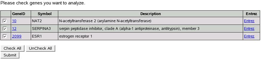
|
At this point our database is searched for all the genes submitted
and figure shows the list of genes found.
Now we can proceed as explained in the previous section ``Search
for genes of interest using entrez id, symbol or description''.
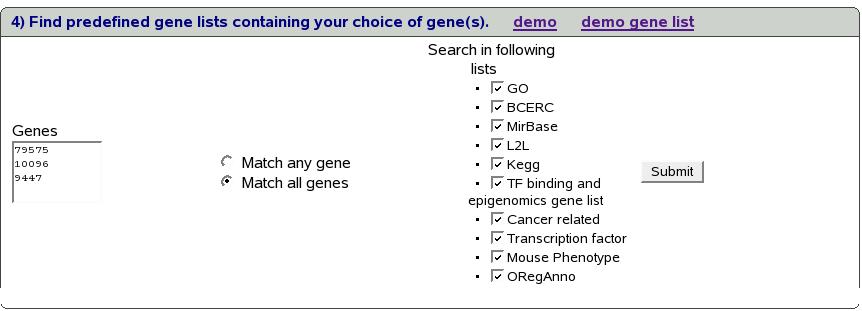
This section describes how to find predefined gene lists that contain
genes of interest.
Figure:
Find predefined gene lists

|
There are two links beside title ``demo'' and ``demo gene list''.
Clicking on demo gene list link shows a few sample genes that we are
going to use for the purpose of this demo. The demo genes are as follows:
79575
10096
9447
Now copy and paste these genes in the text box above. The radio buttons
provide option of how we want to search for the gene lists in the
database. ``Match any gene'' would find all the gene lists that
contain any of the genes we input whereas ``Match all genes''
would find only the gene lists that contain all of the genes.
We also have option of selecting which categories of predefined gene
lists to search.
Figure:
Select categories of predefined gene
lists to search
|
Figure shows all the categories of
predefined gene lists that visible after clicking ``Search in following
lists''.
By default all the lists are selected.
Let's proceed with our example using ``Match all genes'' option
and default case for searching lists (search all lists).
Figure:
Result for finding predefined gene
lists

|
Figure shows the result of our query.
It shows all the gene lists found along with their description.
Let's select first list (NFkB) and submit.
Figure:
Summary of gene list
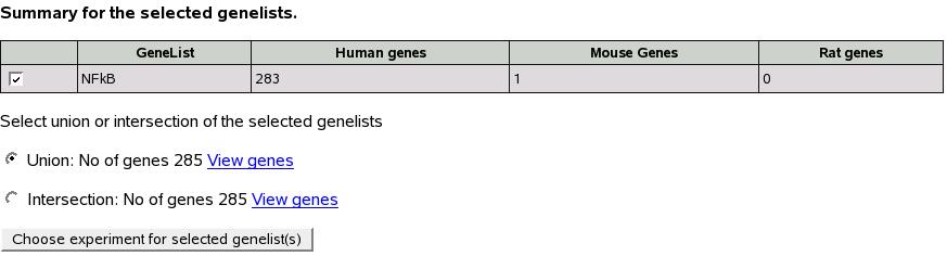
|
Figure shows the resultant screen
which shows the summary of gene lists selected. You might recall that
this is similar to the screen shown in first section ``Using
predefined gene lists'' and rest of the analysis is as described
in that section.
Find genes with a phrase in their
RIFs.
This section describes how to find genes based on their RIFs.
Figure:
Find genes from their RIFs

|
The figure is self-explanatory. Let's
type ``argyrophilic grain disease'' in the box and click submit.
Figure:
RIF search result

|
Figure shows the result of our search.
Select genes of interest and submit. Now we are presented a screen
to select an experiment for analysis. Proceed as explained in previous
section "Search for genes of interest
using entrez id, symbol or description".
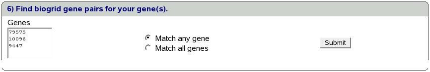
Find biogrid gene pairs for your gene(s).
This section describes how to find biogrid gene pairs for your genes.
Figure:
BioGrid
|
Let's use genes 79575,10096,9447 we used in previous examples. Select
``Match any genes'' option and click submit.
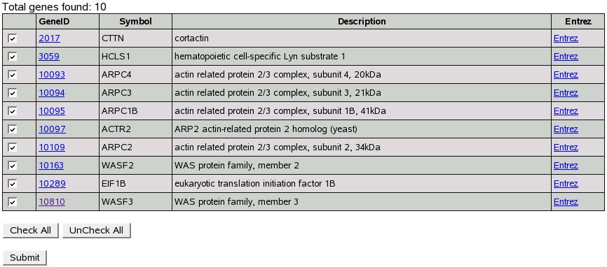
Figure:
BioGrid search result
|
Figure shows result for our search.
Click submit and proceed with analysis as explained in section "Search
for genes of interest using entrez id, symbol or description".
Start by selecting an experiment
If one is interested in a particular experiment, it is useful to locate
the experiment first and then proceed with the analysis.
This section describes how to do this. At the time of this writing,
there are 1904 experiments in the database and this number is continuously
growing. Experiments are organized into different portals. If we know
the portal the experiment of our interest belongs to, we can click
on the portal name to list all the experiments in that portal. Since
this is not the case most times, a search function is provided to
look for experiments of our interest.
Start by clicking ``Experiments'' tab on the left menu.
Figure:
Experiments tab
|
Figure shows the experiment tab. The ``Filter
experiments'' box on top provides search functionality.
The table below shows various portals and their descriptions. Clicking
on a portal name shows the experiments belonging to that portal.
Search for an experiment
Search is a very important part of this portal given the number of
experiments we have. To locate experiments of interest, a simple and
effective search functionality is provided.
Figure:
Search for experiments

|
Figure shows the screen to filter
experiments.
Following are the components of this module:
1) Organism: Experiments could be filtered by selecting one of the
organism from the combo box named ``organism''.
Three options proved are human, mouse and rat.
2) Sample type: Three sample types are provided for selection. Tissue,
cell line and motif score. Select appropriate from the combo box.
3) Data type: Six data types are available for selection from the
combo box.
4) Portal: All the available portals are listed here. Select a portal
if you want to limit your search to that particular portal.
5) Keyword: This could be a name of experiment, a word in description
or reference.
Let's search for experiments with keyword ``miller'' across all
organisms, sample types and portals as an example.
Figure:
Filter experiment result

|
Figure shows a part of the result
page. As shown above, all the experiments found for the search criteria
are listed in a table. Notice the ``Query'' and ``Cluster''
buttons in the last two columns of the table. These buttons provide
a way to analyze the experiments and are explained in detail in following
sections.
Query experiment
Clicking ``Query'' button shown in figure
opens a new window for that particula experiment.
Figure:
Query experiment

|
e.g. Figure shows the query page for experiment
``GSE1045'' in portal Breastcancer. The top table provides a summary
of the experiment and bottom table lists all the properties (sample
subgroupings) available for this experiment. These are useful for
analysis.
These two tables are followed by all the options to construct a gene
list shown in ``Gene List'' tab.
The procedure for analysis is similar to what was described in section
``Start by constructing gene list''
except that the step to select experiment is skipped as we already
have an experiment to work with.
Cluster experiment
Clicking ``Cluster'' button shown in figure
opens a new window for that particular experiment.
Figure:
Cluster experiment
|
Miscellaneous modules
Filter samples and select sample grouping
for analysis
Note: This step is optional and default is to select all the available
samples for analysis.
An experiment may have a number of samples which are organized in
different groups (sample subgroupings).
One may wish to restrict analysis only to a subset of all the available
samples for an experiment.
This section describes how this is achieved.
Figure:
Select samples for analysis

|
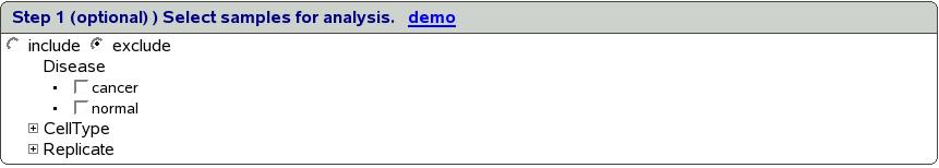
Figure shows the screen to filter samples
for experiment GSE10797. We can choose to either include or exclude
all the samples that satisfy the criteria we are going to define by
selecting appropriate option using the radio button.
All the sample subgroupings are listed in this box. When we click
on a sample subgrouping, the link expands to show all the unique values
for the same as shown in figure .
Figure:
Sample selection expanded
|
Let's say, we want to include only the samples for which Disease is
cancer and CellType is epithelial.
Figure:
Filter sample example

|
As shown in figure , select include
from the radio button, and check cancer box under Disease and epithelial
box under CellType. When you click Analyze, only the samples for this
criteria will be used for analysis.
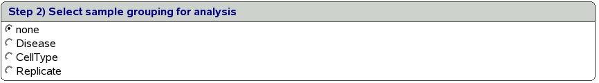
Next step is to select sample grouping for analysis.
Figure:
Select sample group
|
Interpreting Results
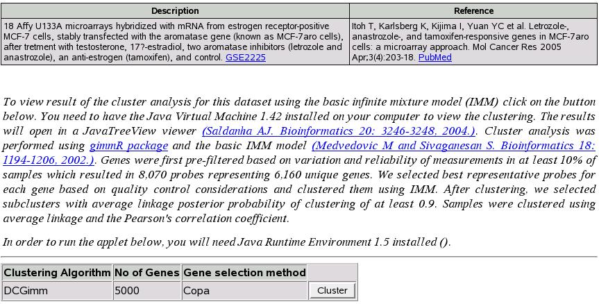
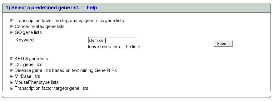
This section will describe the results page in detail. For illustration
purpose we will take all genes with ``stem cell'' keyword in GO
category as shown in figure .
Figure:
Select gene list with ``stem
cell'' keyword
|
Check all the genelists on the resultant page and proceed as explained
in section 'Using predefined gene list(s)'. Select experiment ``GSE2225''
in portal ``Breast cancer'' and use sample subgrouping ``Treatment''
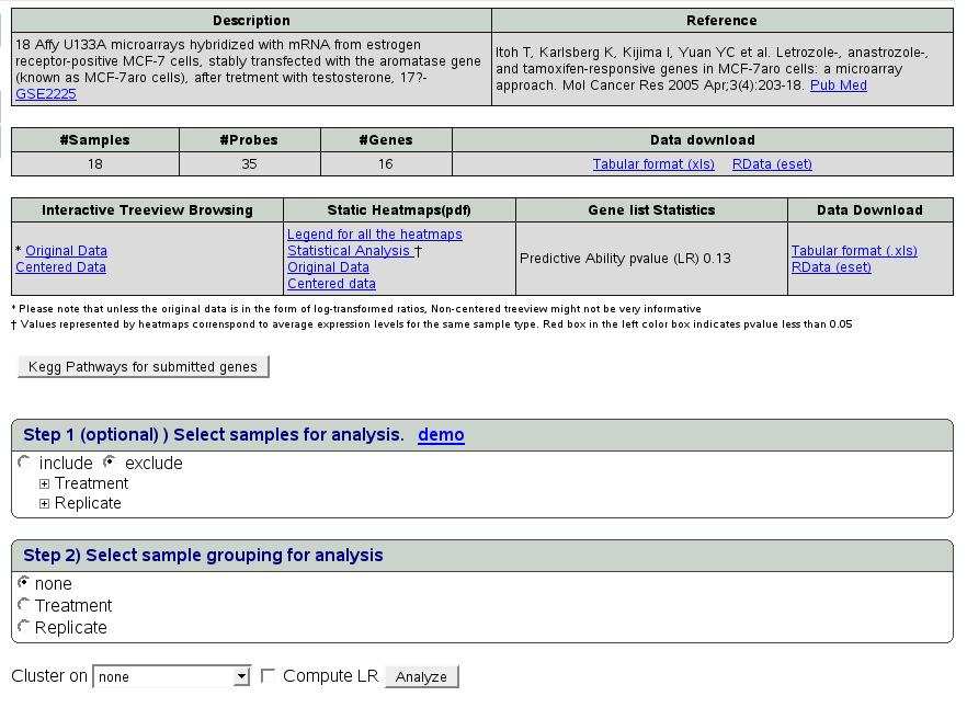
and cluster on ``genes'' to obtain the results shown in figure
.
Figure:
Results of stem cell gene list
query
|
The results page structure is as follows. The first table gives a
brief description of the selected experiment. The second table summarizes
the data retrieved for the analysis of submitted query gene list and
provides links for download. Data can be retrieved in the form of
spreadsheet and R data object. The third table gives the analysis
results which are explained in detail as follows.
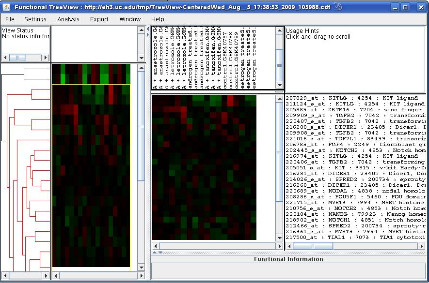
Interactive Treeview Browsing
Unsupervised clustering of the query data was performed using the
Bayesian model-based procedures [1] as well as simple hierarchical
clustering. The functional annotation of the clustering structures
was performed using the CLEAN framework [2], the integrative
browsing of the data and functional annotations is facilitated through
the Functional TreeView (FTreeView) which is a Java web-start based
clustering browser [2]. Using FTreeView, one can identify
clusters of genes based on their data profile and correlation with
specific functional categories and use such gene lists to query and
analyzed genomics data in other datasets.
Figure:
TreeView
|
We would like to note that in the case where no clustering option
(on the genes as well as samples) is chosen, the TreeView application
would show the heatmap with no dendrograms on either sides. This might
make the heatmap incomprehensible at first. However, one can click
on any of the genes or group of genes and the corresponding gene annotations
will be displayed in the rightmost window. The scenario is depicted
in where genes and samples
are not clustered.
Figure:
TreeView with no clustering
of genes and samples

|
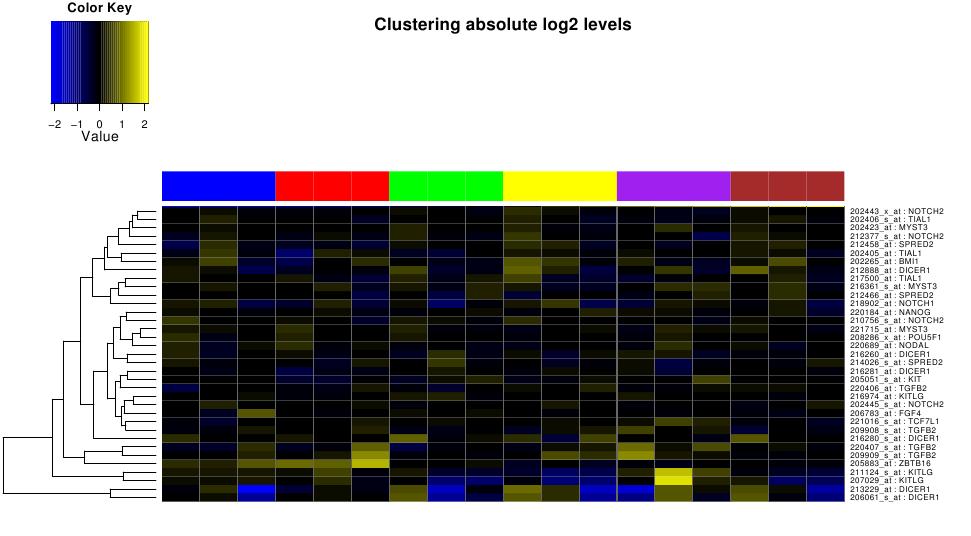
Static heatmaps
In addition to interactive treeview interface, Cluster analysis results
are also available as static annotated heatmaps saved in pdf files.
The values represented by heatmaps correspond to log transformed ratios.
Figure:
Static heatmap for stem cell
genes
|
Figure illustrates static heatmap
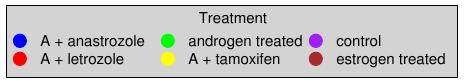
clustered on selected stem cell genes across 6 treatment types. These
sample annotations are provided separately in the link ``legend
for all the heatmaps'' as shown in figure .
Figure:
legend for 6 treatment types
|
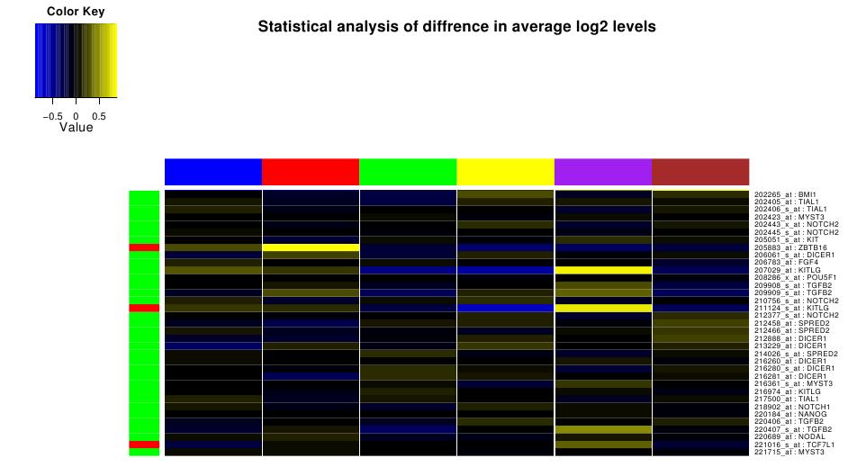
Statistical Analysis
For the selected samples in the dataset, we can identify differentially
expressed significant genes. Values represented by heatmaps correnspond
to average expression levels for the same sample subgrouping. Red
box in the left sidebar indicates pvalue less than 0.05.
Figure:
Statistical Analysis of
stem cell genes
|
Gene List Statistics
Predictive Ability Pvalue (LR)
To assess the predictive ability of the selected sample grouping (in
this exmample ``treatment''), we select random genes of the same
length as that of query gene list from the particular platform. The
enrichment of the statistically significant genes in the query list
was then assessed using logistic regression [3].
Kegg Pathways for submitted genes
Query gene lists are incorporated into KEGG pathway images. One can
click on a Pathway ID to view graphical representation of the pathway.
Significantly expressed genes are painted yellow and other genes that
were found in that particular pathway but are not significantly expressed
are painted blue.
Case Study: Characterizing experimentally
identified proliferation signature
We demonstrate the utility of the Genomics Portals through a case
study investigating proliferation gene expression signature in rat
mammary epithelium induced by different fatty acid diets [4].
This study established the increased proliferation of mammary epithelium
as a consequence of several different dietary regiments in virgin
female Spraque-Dawley rats. The study also identified a set of 85
genes whose expression levels were correlated with the increased proliferation.
We used Genomics Portals to study the functional importance of these
85 genes in five different biological processes examined in 4 gene
expression datasets [5,6,7,8] which are available
in the portal. Here, we present step-by-step instructions for reproducing
the results using Miller et.al. [5] dataset which comprises
of 251 primary human breast tumors. This dataset was re-processed
and curated before being deposited into the back-end databases under
the id ``GSE3494Entrez''. The comparison
of interest in this case was between the largest (top quartile) and
smallest (bottom quartile) tumor with the assumption that large tumors
are ``more proliferative'' than
small tumors.
Go to ``Experiments'' tab and type 'GSE3494Entrez' in the keyword
field of 'Filter experiments' option. You can also find this experiment
under 'Breast Cancer' portal. Press ``submit''. This will fetch
the corresponding experiment and then press ``Query'' button.
Paste a list of Entrez ids of 85 up regulated proliferation genes
found at http://eh3.uc.edu/documentation/upregulatedDietsGenes.txt
in the box (option 3) and press ``submit''.
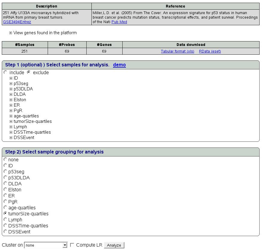
This page provides collective information about the selected dataset,
gene list submitted (and the actual number of probes found on this
platform) as well as sample groupings associated with this dataset.
In this example, select ``tumorSize-quartiles'' as sample grouping
in step 2. We do no want to filter any samples hence we can skip step
1. Also, select ``computeLR'' and press ``Analyze'' button.
Figure depicts the
snapshot of this step.
Figure:
Proliferation genes
on Miller dataset
|
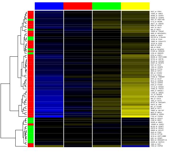
Click on the ``statistical Analysis'' link and you will get a
heatmap as shown in . The
corresponding legends can be found by clicking on the link ``legend
for all the heatmaps'' as shown in .
One can see that indeed the genes in the query list are up-regulated
in large tumors (quart-4) and are enriched for differentially expressed
gene (LRpath p-value<10-9).
Figure:
Legend for Tumor Size grade

|
Figure:
Statistical significance
of up regulated genes
|
Similar analysis could be performed on the other 3 datasets using
the same list of 85 up regulated proliferation genes. We have established
the universality of the proliferation signature identified in the
rat dietary studies across four very different biological systems
using the Genomics Portals interface. The entire process of querying
and generating results can be completed in less than 10 minutes. More
details could be obtained from the manuscript.
In addition to using gene expression data, we further characterize
our proliferation signature using ChIP-seq data for E2F1 transcription
factor (TF) [9]. In the original paper, an extended set
of genes identified through cluster analysis was linked to regulatory
domain of E2F transcription factors by examining the overlap with
E2F targets established in ChIP-chip [10] and global expression
profiling [11] experiments, and computationally predicted
E2F targets. Here, we used Genomics Portals to examine the newer ChIP-seq
dataset assessing DNA binding of 15 different transcription factors,
including E2F1, in mouse embryonic stem cells. Following steps can
be conducted to obtain the respective heatmaps.
Go to ``Experiments'' tab and type 'GSE11431peaks' in the keyword
field of 'Filter experiments' option. You can also find this experiment
under 'Transcription Factors' portal. Press ``submit''. This will
fetch the corresponding experiment and then press ``Query'' button.
Paste a list of Entrez ids of 85 up regulated proliferation genes
in the box (option 3) and press ``submit''.
Select ``Transcriptionfactor'' as sample grouping in step 2. We
do no want to filter any samples hence we can skip step 1 and then
press ``Analyze''
Click on the link ``Centered data'' under static heatmap column
of the result table. Figure shows heatmap
of 15 Tfs and figure displays corresponding
legends for each of the TFs.
Figure:
Legend for 15 TFs

|
Figure:
Heatmap of 15 TFs

|
We can see that in addition to most of the genes having a ChIP-seq
peak for E2F1 within the regulatory region examined (-4kb to +1kb
around TSS marked by 0), there were several other transcription factors
such as N-myc,Tcfp2l1,c-Myc etc. that seem to have unusually many
peaks for these gene. We can then focus on each of the TFs separately
to take a closer look. We will illustrate the case using n-Myc TF.
We can select n-Myc TF out of 15 Tfs using ``select sample'' option
in step 1 as shown in figure . Expand ``Transcription
Factor'' and select n-Myc TF and click radio button ``include''
to select this sample. Then select ``TranscriptionFactor'' in
step 2. select Cluster on ``Genes'' and ``compute LR'' options
and click ``Analyze''.
Figure:
Select n-Myc TF

|
Then click on the link ``Centered data'' under static heatmap
column of the result table. Figure shows
increased binding around TSS of the promoter region (-4kb to +1kb
in this case) for some of these genes.
Figure:
n-Myc TF heatmap

|
Here, we used the comparison to ``random''
sample by LRpath. Instead of the p-values, in this situation Genomics
Portals by default uses the maximum ``peak intensity''
calculated for each gene across its whole regulatory region. Such
statistical analysis confirmed that in addition to E2F1 (p-value <
10-14), n-Myc (p-value < 10-7), Tcfp2l1 (p-value < .001), c-Myc (p-value
< .01), and Klf4 (p-value < 0.01) all show signs of increased binding
to regulatory regions of these genes.
We performed similar analysis on two epigenomics histone marks, H3k4me3
and H3k27me3 across five human cell line at different ``differentiation''
stages [12]. Following steps can be conducted to obtain
the respective heatmaps.
Go to ``Experiments'' tab and type 'GSE11074' in the keyword field
of 'Filter experiments' option. You can also find this experiment
under 'Epigenomics' portal. Press submit. This will fetch the corresponding
experiment and then press ``Query'' button.
Paste a list of Entrez ids of 85 up regulated proliferation genes
in the box (option 3) and press ``submit''.
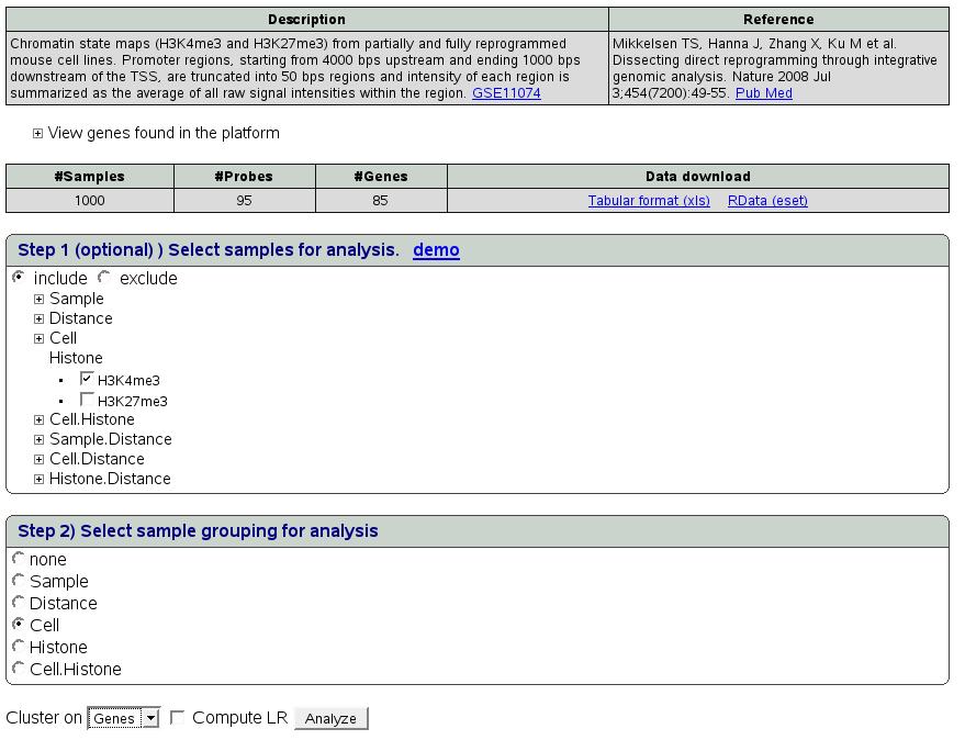
In step1 (select samples for analysis), click on sample grouping name
'Histone'. This will show 2 options namely H3k4me3 and H3K27me3. We
want to analyze the 2 histones separately. Choose H3K4me3 first by
checking radio button 'include'. This step will filter samples in
the analysis. In this case it will include only one type of selected
histone. In step2, select ``cell'' as sample grouping for further
analysis. Then choose clustering on ``Genes'' and press ``Analyze''.
Figure depicts the snapshot of this
step.
Figure:
Filter H3k4me3 histone samples
|
Click on ``Centered data'' link in the static heatmap column of
the summary results table. Similar steps could be performed for other
histone type. Figure and figure
show heatmaps of the 2 histones
respectively. Figure shows legend for 5 cell
types.
Figure:
Legend for 5 cell types

|
Figure:
Histone H3k4me3 Heatmap

|
Figure:
Histone H3k27me3 Heatmap

|
The results indicate that there is a subset of genes is in our proliferation
signature with strong tri-mehylation of histone 3's
lysine 4 across all 5 cell lines. On the other hand, tri-methylation
of histone 3's lysine 27, in addition for differences
between genes, also shows differences between different cell lines.
- 1
- Liu X, Sivaganesan S, Yeung KY, Guo J, Bumgarner RE,
Medvedovic M: Context- specific infinite mixtures for clustering gene
expression profiles across diverse microarray dataset. Bioinformatics
2006, 22:1737-1744.
- 2
- Freudenberg JM, Joshi VK, Hu Z, Medvedovic M: CLEAN:
CLustering Enrichment ANalysis. BMC Bioinformatics 2009, 10:234.
- 3
- Sartor MA, Leikauf GD, Medvedovic M: LRpath: A logistic
regression approach for identifying enriched biological groups in
gene expression data 2. Bioinformatics 2008.
- 4
- Medvedovic M, Gear R, Freudenberg JM, Schneider J,
Bornschein R, Yan M, Mistry MJ, Hendrix H, Karyala S, Halbleib D et
al.: Influence of Fatty Acid Diets on Gene Expression in Rat Mammary
Epithelial Cells. Physiol Genomics 2009.
- 5
- Miller LD, Smeds J, George J, Vega VB, Vergara L,
Ploner A, Pawitan Y, Hall P, Klaar S, Liu ET et al.: From The Cover:
An expression signature for p53 status in human breast cancer predicts
mutation status, transcriptional effects, and patient survival. PNAS
2005, 102:13550-13555.
- 6
- Fournier MV, Martin KJ, Kenny PA, Xhaja K, Bosch I,
Yaswen P, Bissell MJ: Gene Expression Signature in Organized and Growth-Arrested
Mammary Acini Predicts Good Outcome in Breast Cancer. Cancer Res 2006,
66:7095-7102.
- 7
- Herschkowitz J, Simin K, Weigman V, Mikaelian I, Usary
J, Hu Z, Rasmussen K, Jones L, Assefnia S, Chandrasekharan S et al.:
Identification of conserved gene expression features between murine
mammary carcinoma models and human breast tumors. Genome Biology 2007,
8:R76.
- 8
- Moggs JG, Murphy TC, Lim FL, Moore DJ, Stuckey R,
Antrobus K, Kimber I, Orphanides G: Anti-proliferative effect of estrogen
in breast cancer cells that re- express ER{alpha} is mediated by
aberrant regulation of cell cycle genes. J Mol Endocrinol 2005, 34:535-551.
- 9
- Chen X, Xu H, Yuan P, Fang F, Huss M, Vega VB, Wong
E, Orlov YL, Zhang W, Jiang J et al.: Integration of External Signaling
Pathways with the Core Transcriptional Network in Embryonic Stem Cells.
Cell 2008, 133:1106-1117.
- 10
- Xu X, Bieda M, Jin VX, Rabinovich A, Oberley MJ,
Green R, Farnham PJ: A comprehensive ChIP-chip analysis of E2F1, E2F4,
and E2F6 in normal and tumor cells reveals interchangeable roles of
E2F family members. Genome Res 2007, 17:1550-1561.
- 11
- Kalma Y, Marash L, Lamed Y, Ginsberg D: Expression
analysis using DNA microarrays demonstrates that E2F-1 up-regulates
expression of DNA replication genes including replication protein
A2 3. Oncogene 2001, 20:1379-1387.
- 12
- Mikkelsen TS, Hanna J, Zhang X, Ku M, Wernig M, Schorderet
P, Bernstein BE, Jaenisch R, Lander ES, Meissner A: Dissecting direct
reprogramming through integrative genomic analysis 2. Nature 2008,
454:49-55.